CNN-based Handwritten Digit Recognition

from __future__ import absolute_import, division, print_function, unicode_literals

# TensorFlow and tf.keras
import tensorflow as tf
from tensorflow import keras
from tensorflow.keras import backend as K

# Helper libraries
import numpy as np
import matplotlib.pyplot as plt
import random

print(tf.__version__)

Import MNIST dataset

This guide uses the MNIST dataset which contains 70,000 grayscale images in 10 categories. MNIST stands for Mixed National Institute of Standards and Technology database.
The MNIST dataset is often used as the “Hello, World” of machine learning programs for computer vision. It contains images of handwritten digits (0, 1, 2, etc.).
Here, 60,000 images are used to train the network and 10,000 images to evaluate how accurately the network learned to classify images. You can access MNIST directly from TensorFlow. Import and load MNIST data directly from TensorFlow:

mnist = keras.datasets.mnist

(train_images, train_labels), (test_images, test_labels) = mnist.load_data()

# grayscale image has only 1 channal
if K.image_data_format() == 'channels_first':
    train_images = train_images.reshape(train_images.shape[0], 1, 28, 28)
    test_images = test_images.reshape(test_images.shape[0], 1, 28, 28)
    input_shape = (1, 28, 28)
else:
    train_images = train_images.reshape(train_images.shape[0], 28, 28, 1)
    test_images = test_images.reshape(test_images.shape[0], 28, 28, 1)
    input_shape = (28, 28, 1)

Explore the data

Let’s explore the format of the dataset before training the model. The following shows there are 60,000 images in the training set, with each image represented as 28 x 28 pixels:

1 2	train_images.shape #out:(60000, 28, 28, 1) #the shape of the trainset

1
2
3

#Likewise, there are 60,000 labels in the training set:
len(train_labels)
#out:60000

1
2
3

#Each label is an integer between 0 and 9:
train_labels
#out:array([5, 0, 4, ..., 5, 6, 8], dtype=uint8)

1
2
3

#Each label is an integer between 0 and 9:
test_images.shape
#out:(10000, 28, 28, 1)

1
2
3

#And the test set contains 10,000 images labels:
len(test_labels)
#out:10000

Preprocess the data

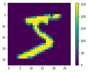
The data must be preprocessed before training the network. If you inspect the first image in the training set, you will see that the pixel values fall in the range of 0 to 255:

plt.figure()
plt.imshow(train_images[0,:,:,0])#choose the first one in the set
plt.colorbar()
plt.grid(False)#no grid line #plt.grid(linestyle=":", color="r")
plt.show()

Scale these values to a range of 0 to 1 before feeding them to the neural network model. To do so, divide the values by 255. It’s important that the training set and the testing set be preprocessed in the same way.
In addition, encode labels using one-hot encoding.

train_images_normed = train_images / 255.0 #make the value between 1 and 0

test_images_normed = test_images / 255.0

train_labels_onehot = keras.utils.to_categorical(train_labels, 10)

test_labels_onehot = keras.utils.to_categorical(test_labels, 10)

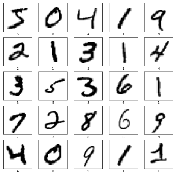
To verify that the data is in the correct format and that you’re ready to build and train the network, let’s display the first 25 images from the training set and display the class name below each image.

plt.figure(figsize=(10,10))
for i in range(25): #choose 25 sample and put them in 5x5 graph
    plt.subplot(5,5,i+1)
    plt.xticks([])
    plt.yticks([])
    plt.grid(False)
    plt.imshow(train_images[i,:,:,0], cmap=plt.cm.binary)
    plt.xlabel(train_labels[i])
plt.show()

Build the model

Building the neural network requires configuring the layers of the model, then compiling the model.
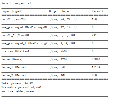
This example is LeNet-5, you can modify the model as you like.

model = keras.Sequential([
    keras.layers.Conv2D(6, kernel_size=(5, 5),
                 activation='relu',
                 input_shape=input_shape),
    keras.layers.MaxPooling2D(pool_size=(2, 2)),
    keras.layers.Conv2D(16, kernel_size=(5, 5), activation='relu'),
    keras.layers.MaxPooling2D(pool_size=(2, 2)),
    keras.layers.Flatten(),
    keras.layers.Dense(120, activation='relu'),
    keras.layers.Dense(84, activation='relu'),
    keras.layers.Dense(10, activation='softmax')
])

Observe the summary.

1	model.summary()

Define the process you train the model.

1
2
3

model.compile(loss=keras.losses.categorical_crossentropy,
              optimizer=keras.optimizers.Adam(),
              metrics=['accuracy'])

Train the model

Feed the model

To start training, call the model.fit method—so called because it “fits” the model to the training data:

1 2	model.fit(train_images_normed, train_labels_onehot, batch_size=100, epochs=6) # It may need more than one minute

As the model trains, the loss and accuracy metrics are displayed.

Evaluate accuracy

Next, compare how the model performs on the test dataset:

1
2
3

test_loss, test_acc = model.evaluate(test_images_normed, test_labels_onehot, verbose=2)

print('\nTest accuracy:', test_acc)Make predictions

Make predictions

1	predictions = model.predict(test_images_normed)

Here, the model has predicted the label for each image in the testing set. Let’s take a look at the first prediction:

1	predictions[0]

A prediction is an array of 10 numbers. They represent the model’s “confidence” that the image corresponds to each of the 10 different articles of clothing. You can see which label has the highest confidence value:

1 2	np.argmax(predictions[0]) #out:7

So, the model is most confident that this image is 7. Examining the test label shows that this classification is correct:

1 2	test_labels[0] #out:7

Graph this to look at the full set of 10 class predictions.

def plot_image(i, predictions_array, true_label, img):
    predictions_array, true_label, img = predictions_array, true_label[i], img[i,:,:,0]
    plt.grid(False)
    plt.xticks([])
    plt.yticks([])

    plt.imshow(img, cmap=plt.cm.binary)

    predicted_label = np.argmax(predictions_array)
    if predicted_label == true_label:
        color = 'blue'
    else:
        color = 'red'

    plt.xlabel("Pred:{} {:2.0f}% (GT:{})".format(predicted_label,
                                100*np.max(predictions_array),
                                true_label),
                                color=color)

def plot_value_array(i, predictions_array, true_label):
    predictions_array, true_label = predictions_array, true_label[i]
    plt.grid(False)
    plt.xticks(range(10))
    plt.yticks([])
    thisplot = plt.bar(range(10), predictions_array, color="#777777")
    plt.ylim([0, 1])
    predicted_label = np.argmax(predictions_array)

    thisplot[predicted_label].set_color('red')
    thisplot[true_label].set_color('blue')

Verify predictions

With the model trained, you can use it to make predictions about some images.

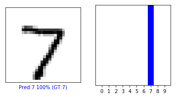
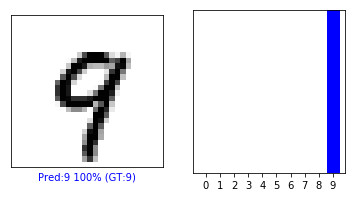
Let’s look at the 0th image, predictions, and prediction array. Correct prediction labels are blue and incorrect prediction labels are red. The number gives the percentage (out of 100) for the predicted label.

i = 0
plt.figure(figsize=(6,3))
plt.subplot(1,2,1)
plot_image(i, predictions[i], test_labels, test_images)#show the original one
plt.subplot(1,2,2)
plot_value_array(i, predictions[i],  test_labels)#show the predicted one
plt.show()

i = 12
plt.figure(figsize=(6,3))
plt.subplot(1,2,1)
plot_image(i, predictions[i], test_labels, test_images)
plt.subplot(1,2,2)
plot_value_array(i, predictions[i],  test_labels)
plt.show()

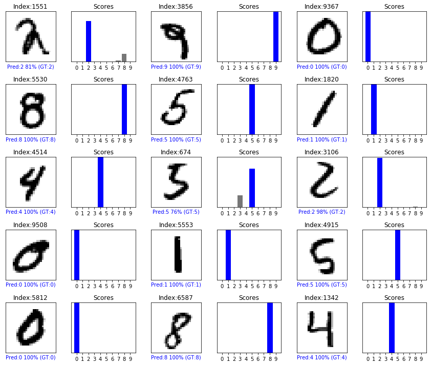
Let’s plot several images with their predictions. Note that the model can be wrong even when very confident.

# Plot random 25 test images, their predicted labels, and the true labels.
# Color correct predictions in blue and incorrect predictions in red.
h = set()
while(len(h)<25):
    h.add(random.randint(0, 9999))
    
num_rows = 5
num_cols = 3
num_images = num_rows*num_cols
plt.figure(figsize=(2*2*num_cols, 2*num_rows))
i = 0
for p in h:
    plt.subplot(num_rows, 2*num_cols, 2*i+1)
    plot_image(p, predictions[p], test_labels, test_images)
    plt.title("Index:{}".format(p))
    plt.subplot(num_rows, 2*num_cols, 2*i+2)
    plot_value_array(p, predictions[p], test_labels)
    plt.title("Scores")
    i = i + 1
    if i >= 15:
        break
plt.tight_layout()
plt.show()